Freeway – Corridor Traffic Plotting
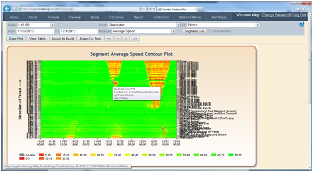
Corridor traffic plotting is designed to present traffic conditions of long stretch of freeway over a certain time period on one graph (contour plot). Large amount of spatial and temporal traffic information can be viewed at the same time. Traffic pattern, trend, bottleneck, congestion level, crashes, and impact of crashes can be easily observed. For example, the screenshot below clearly shows the 2013 Thanksgiving holiday traffic on I-15 SB between Las Vegas and the California stateline. On high-volume outbound days, congestion occurs because capacity of the freeway is reduced in California. On this particular weekend, travelers experienced a 33-mile queue on Sunday, December 1st.
Corridor, origination and destination, date range, and measures are user customizable. And the measures include average speed, average lane volume, HOV or express lane speed and volume, general purpose lane speed and volume.
How to use:
1. Select corridor, the origination and destination, date range, measure type from the top panel.
2. Click “Draw Plot” to show the contour plot; Click “View Table” to show the corresponding data; Click “Export to Excel” or “Export to Text” to download the data in Excel or Text format.
3. If there an incident on the selected corridor and within the time range, incident icon will appear on the plot. User can click the incident icon to open a popup window to show the histocial traffic animation and camera snapshots (accessible to approved user only).
4. User can click on the "<<", "<", ">", ">>" to draw the plot of the same day of the previous/next week or month to compare the plots and see the pattern.
Note:
· If the selected date range is too long, it may take a while to generate the plot. If error happens while loading the plot, please select shorter date range.
· To view the selected segments, please click on the “Segment List”.
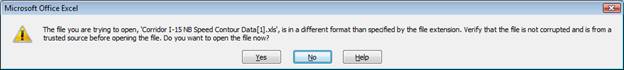
· When open the exported Excel file, Excel 2007 will prompt a warning message as shown in the figure below. You may ignore this message and click “Yes” to open this file.
How to read the plot:
1. The X-axis is the time series. The granularity is 15-minute slice;
2. The Y-axis is the sequence of selected segments. The direction of travel is from the bottom to the top. You may use the “Segment List” as a look-up table to see the segment location;
3. The selected measure is colorized according to the legend on the bottom.